Mediation analysis is a simple idea that is easy to do, but an absolute minefield to interpret correctly. The principal is easy – perhaps one explanatory variable correlates with the dependent variable by mediating (effecting) an other explanatory variable. So say you find out that bullet wounds correlates with death and blood loss correlates with death, you could do a mediation analysis to see if bullet wounds correlates with death by affecting blood loss – and you would find that it does (sorry about the gruesome example). One absolute NO NO for mediation analyses is if the direction of causation could be the other way. i.e. the dependent variable causes the explanatory variables. All mediation analyses breaks down at this point, so don’t do it (cough – like this paper did – https://pubmed.ncbi.nlm.nih.gov/29567761/ – cough). For example if you modelled bullet wounds as the dependent variables and explained it with death and blood loss as a mediation factor, you would find that death causes bullet wounds directly and indirectly through blood loss. This obviously doesn’t make sense (this is different to just correlation analyses that doesn’t care about the direction of causality).

In this example we are seeing whether or not the age of a patient correlates with inflammation through the variable bacterial count. The idea being that being old not only directly causes inflammation, but perhaps makes you more susceptible to bacteria growth, leading to larger numbers of bacteria in your blood and this leads to more inflammation. Now to make this even more complicated (just because that is how data is) what if you wanted to get rid of some nuisance variables first, before looking at your explanatory variables of interest? Wow, OK, here we go.

First Load the data and packages. Make sure the data makes sense (you should always do this),  e.g. are the numerical variables numerical?

#Load package
library(MASS)
library("mediation")
#Load data
dat<- read.table(url("https://jackauty.com/wp-content/uploads/2020/05/Stepwise-regression-data.txt"),header=T)

#Check data, make sure it makes sense
str(dat)

'data.frame': 100 obs. of 8 variables:
 $ Inflammation : num 4.4 1218.07 5.32 3072.58 108.86 ...
 $ Age : num 7.16 8.88 3.23 7.91 7.98 2.93 9.12 9.41 7.71 2.91 ...
 $ Sex : Factor w/ 2 levels "F","M": 2 1 1 1 2 1 1 2 1 1 ...
 $ Blood.pressure : num 151 145 104 156 143 159 114 140 149 114 ...
 $ Infection : Factor w/ 2 levels "No","Yes": 1 2 1 2 1 1 1 1 2 1 ...
 $ Bacterial.count : num 75 5718 27 4439 224 ...

Next, check if the dependent variable is normally distributed. It doesn’t have to be, but things will go smoother if it is. In this example the dependent variable distribution was improved by a square-root transformation. So I created a new transformed variable.

#Check dependent variable, ideally it's normally distributed. Transform if need
hist(dat$Inflammation, breaks=6)



hist(sqrt(dat$Inflammation), breaks=6)


#Square root looks better, so let's create a variable to use in our model
dat$Inflammation.transformed<-sqrt(dat$Inflammation)

Next let’s build a model with the nuisance variables (Sex and Blood Pressure) and extract the standardized residuals into a new column of our dataframe. Residuals (Standardized) are the left over variation after the accounting for the nuisance variables. This residual variation will then hopefully be mostly explained by our variables of interest. Check the assumptions and transform if needed.

#Set up adjusted model
adjusted.model<-lm(Inflammation.transformed ~ Sex*Blood.pressure, data = dat)
summary(adjusted.model)

#Check Assumptions
par(mfrow=c(2,2))
plot(adjusted.model)



#Extract the standardized residuals and turn them into a column in your data
dat$residuals<-stdres(adjusted.model)

#Check your data
dat[1:20,]

Next let’s build our base models with our two explanatory variables. First with our primary explanatory variable (Age), then with our primary explanatory variable and our mediator variable (Bacterial count). Then check your assumptions. Here it looks like we need to transform our explanatory variable of bacterial count. Often things like bacterial count need a log transformation and it worked!

#Build base models

fit.direct.model<-lm(residuals~Age, data=dat)
fit.mediator.variable.model<-lm(residuals~Age+Bacterial.count, data=dat)
summary(fit.direct.model)
summary(fit.mediator.variable.model)

#Assumption check
par(mfrow=c(2,2)) 
plot(fit.direct.model)
plot(fit.mediator.variable.model)


#Top left you can clearly see the relationship isn't linear.

#Transform predicting variable
dat$log.bacterial.count<-log(dat$Bacterial.count)

fit.direct.model<-lm(residuals~Age, data=dat)
fit.mediator.variable.model<-lm(residuals~Age + log.bacterial.count, data=dat)

summary(fit.direct.model)
summary(fit.mediator.variable.model)

#Assumption check
par(mfrow=c(2,2)) 

plot(fit.direct.model)
plot(fit.mediator.variable.model)


#NNNIIIICCCEEEEE

Now we need to centre the variables. This is important as coefficients are only comparable when the explanatory variables are centred. In this example you might get a small coefficient for bacterial counts, because bacterial counts are in the millions and you might get a large coefficient for Age because that maxes out at 100 (ish). But if you centre both variables (turning them into Z scores), then they become more comparable as they’re on the same scale.

#Centering variables
dat$log.bact.centred<-(dat$log.bacterial.count-mean(dat$log.bacterial.count))/sd(dat$log.bacterial.count)
dat$Age.centred<-(dat$Age-mean(dat$Age))/sd(dat$Age)

Next we get to run our mediation analysis and boomtown we get a significant effect of Age on inflammation and a mediation effect of Age on inflammation through the the effect of age on bacterial count. We ran it again with a boot-strap method that is more robust and less susceptible to a lack of normality in the residuals and we got the same result. Our results show that more than 50% of the effect of Age on inflammation can be explained by bacterial count. This suggests that being elderly increases the risk of a bacterial infection and this explains a good proportion of why the elderly have more inflammation (note this data is made up).

#Running models with centred variables
fit.direct.model.centred<-lm(residuals~Age.centred, data=dat)
fit.mediator.variable.model.centred<-lm(residuals~Age.centred + log.bact.centred, data=dat)



#Run mediation analysis
mediation<-mediate(fit.direct.model.centred, fit.mediator.variable.model.centred, treat="Age.centred", mediator = "log.bact.centred")

summary(mediation)



#Bootsrap method for extra robustness
boot.mediation<-mediate(fit.direct.model.centred, fit.mediator.variable.model.centred, treat="Age.centred", mediator = "log.bact.centred", boot=T, sims=5000)

summary(boot.mediation)

Often you have a truck load of potential explanatory variables, that all might interact with each other, giving a multitude of potential ways the explanatory variables could relate to the dependent variable. You could painstakingly create every possible model or you could do a step-wise regression. Step-wise regression automatically adds and subtracts variables from your model and checks whether it improves the model using AIC as a selection criteria (AIC is a relative score of goodness).

Below is how I would do it. In this example we are trying to explain inflammation with a number of variables such as Age, Sex, Bacterial Count etc.

First Load the data and packages. Make sure the data makes sense (you should always do this),  e.g. are the numerical variables numerical?

#Load package
library(MASS)

#Load data
dat<- read.table(url("https://jackauty.com/wp-content/uploads/2020/05/Stepwise-regression-data.txt"),header=T)

#Check data, make sure it makes sense
str(dat)

'data.frame': 100 obs. of 8 variables:
 $ Inflammation : num 4.4 1218.07 5.32 3072.58 108.86 ...
 $ Age : num 7.16 8.88 3.23 7.91 7.98 2.93 9.12 9.41 7.71 2.91 ...
 $ Sex : Factor w/ 2 levels "F","M": 2 1 1 1 2 1 1 2 1 1 ...
 $ Blood.pressure : num 151 145 104 156 143 159 114 140 149 114 ...
 $ Infection : Factor w/ 2 levels "No","Yes": 1 2 1 2 1 1 1 1 2 1 ...
 $ Bacterial.count : num 75 5718 27 4439 224 ...
 $ Inflammation.transformed : num 2.1 34.9 2.31 55.43 10.43 ...
 $ inflammation.boxcox.transformed: num 2.43 71.02 2.73 123.74 16.68 ...

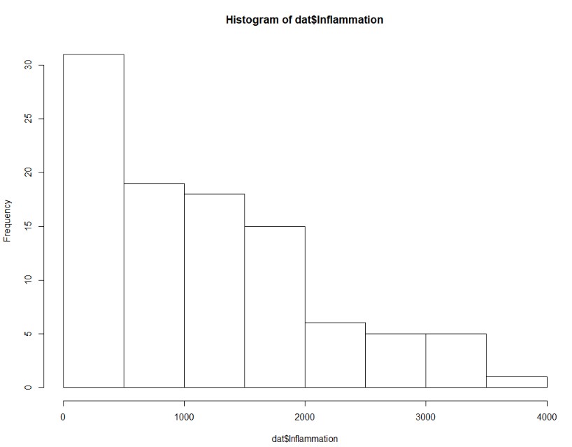
Next, check if the dependent variable is normally distributed. It doesn’t have to be, but things will go smoother if it is. In this example the dependent variable distribution was improved by a square-root transformation. So I created a new transformed variable.

#Check dependent variable, ideally it's normally distributed. Transform if need
hist(dat$Inflammation, breaks=6)



hist(sqrt(dat$Inflammation), breaks=6)


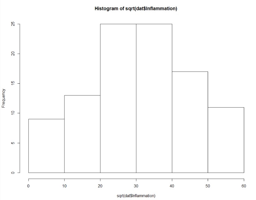#Square root looks better, so let's create a variable to use in our model
dat$Inflammation.transformed<-sqrt(dat$Inflammation)

Next let’s build the full model. The full model is a model with all the explanatory variables interacting with each other! and then run a step-wise regression in both directions (stepping forward and backward)

#Set up full model
full.model<-lm(Inflammation.transformed ~ Age*Sex*Blood.pressure*Infection*Bacterial.count, data = dat)
summary(full.model)


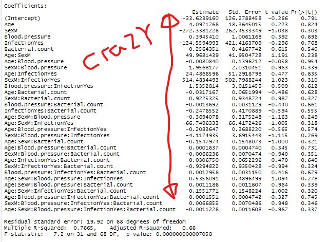#Full model is crazy (note red notes generated in paint :))

#Perform stepwise regression in both directions
step.model<-stepAIC(full.model, direction="both", trace = F)

summary(step.model)

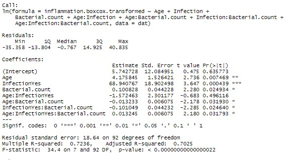
Now given the marginal significance of the three way interaction term, and the difficulty in interpreting three-way interaction terms, I’d be tempted to make a model without that term and check if there is a substantial difference in the model (using AIC or adjusted Rsquared). If the difference is minor, I’d go with the more parsimonious model.

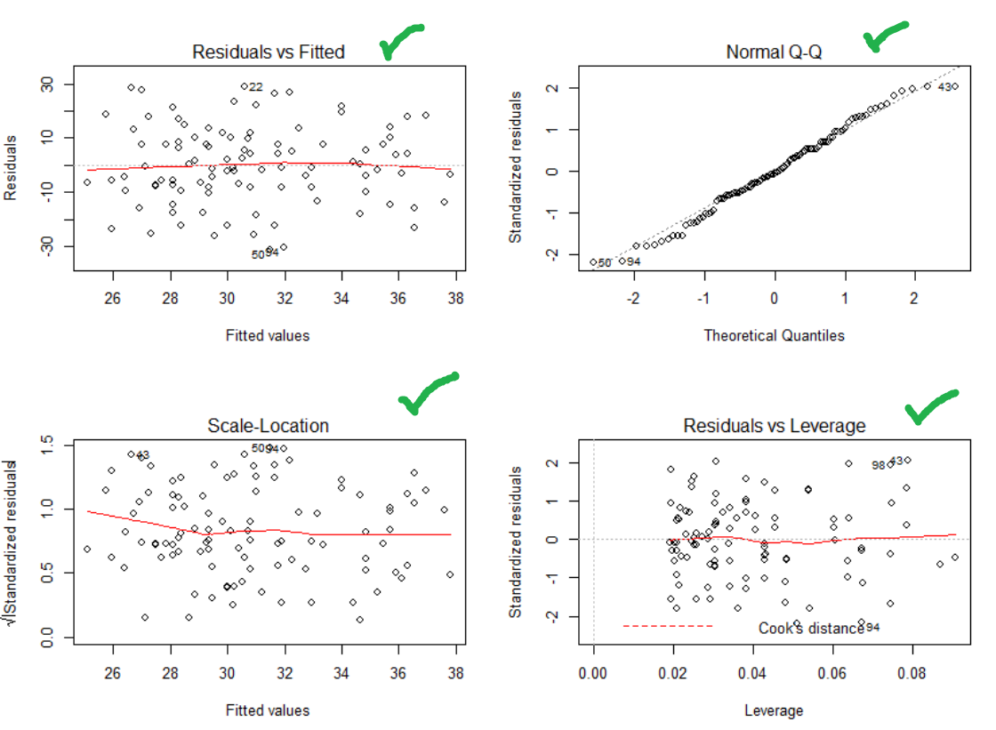
One last step! Check that your residuals are heteroskedastic, normally distributed and there are no major outliers.

#Make it so you can see four graphs in one plot area
par(mfrow=c(2,2)) 

#Plot your assumption graphs
plot(step.model)

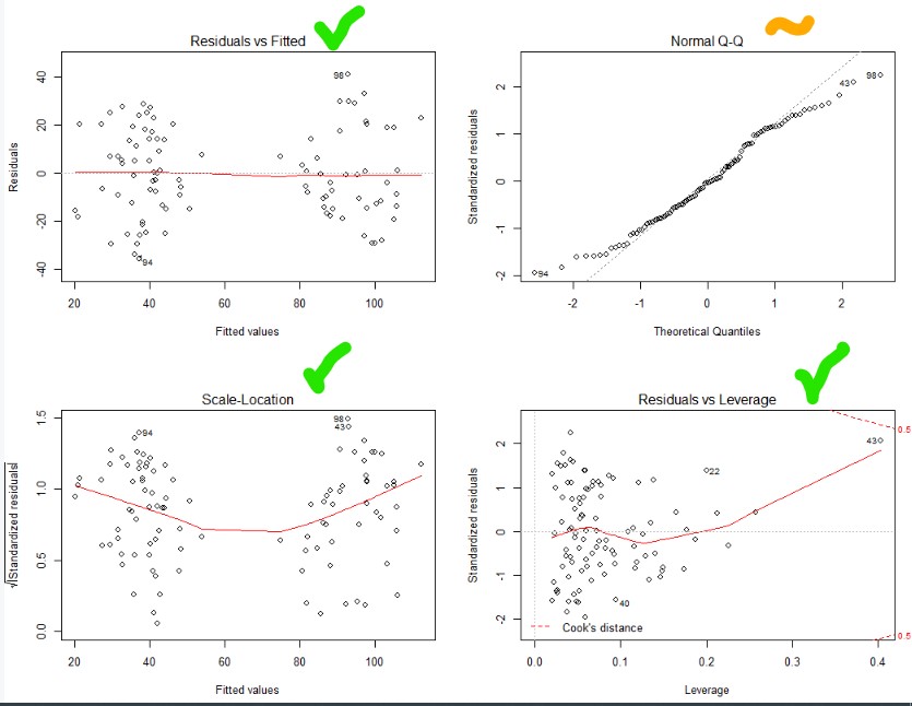
Top and bottom left – nice and flat. Heteroskedastic and no relationship between fitted value and the variability. Nice

Bottom right – no outliers (you’ll see dots outside of the dotted line, if their were)

Top right – ideally all the dots are on the line (normally distributed). So let’s try a better transformation of our dependent variable using a BoxCox transformation!

Box-Cox transformation!

The Box-Cox transformation is where the Box-Cox algorithm works out the best transformation to achieve normality.

First run the stepwise model as above but with the un-transformed variable. Then run the final model through the Box-Cox algorithm setting the potential lamba (power) to between -5 and 5. Lambda is the power that you are going to raise your dependent variable to.

Box-Cox algorithm will essentially run the model and score the normality over and over again. Each time transforming the dependent variable to every power between -5 and 5 going in steps on 0.001. The optimal power is where the normality reaches its maximum. So you then create the variable “Selected.Power” where the normality score was at it’s max. You then raise your dependent variable to that power and run your models again!

#BoxCox transformation
full.model.untransformed<-lm(Inflammation ~ Age*Sex*Blood.pressure*Infection*Bacterial.count, data = dat)
step.model.untransformed<-stepAIC(full.model, direction="both", trace = F)

boxcox<-boxcox(step.model.untransformed,lambda = seq(-5, 5, 1/1000),plotit = TRUE )
Selected.Power<-boxcox$x[boxcox$y==max(boxcox$y)]
Selected.Power
> 0.536

dat$inflammation.boxcox.transformed<-dat$Inflammation^Selected.Power

The Box-Cox algorithm chose 0.536, which is really close to a square-root transformation. But this minor difference does effect the distribution of the residuals.

#Running again with BoxCox transformed variable
#Set up full model
full.model<-lm(inflammation.boxcox.transformed ~ Age*Sex*Blood.pressure*Infection*Bacterial.count, data = dat)

#Perform stepwise regression in both directions
step.model<-stepAIC(full.model, direction="both", trace = F)

summary(step.model)


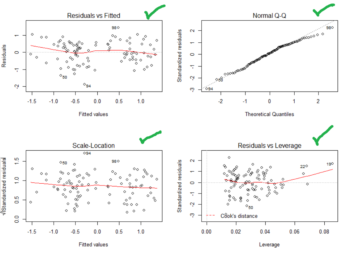
#Checking assumptions 
par(mfrow=c(2,2)) 
plot(step.model)

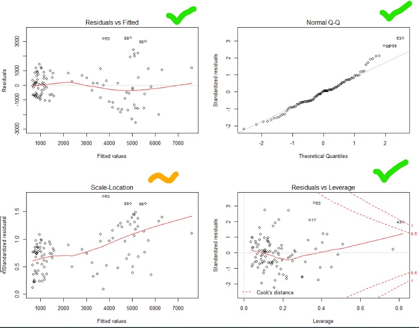
Top right – Yes that is pretty good. Normality achieved!

Top and bottom left – Ok, not great. Things get a bit more variable as the predicted values go up. Guess you can’t win them all.

Bottom right – no outliers beyond the dotted line (1). Though one is close.